Theory Track · Module 10 · Section 2

The Milky Way Galaxy

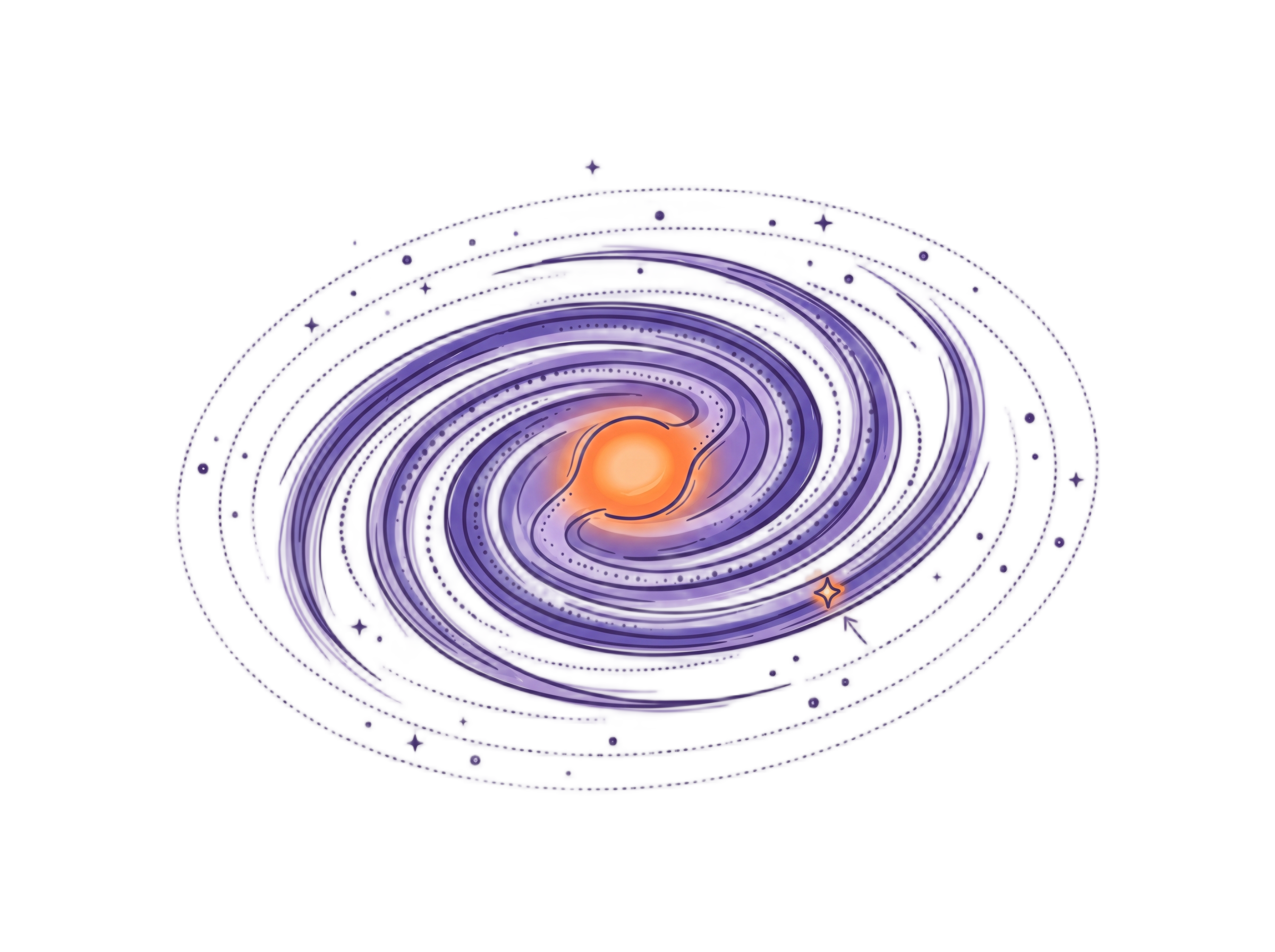
We live inside the Milky Way — a barred spiral galaxy roughly 50 kpc in diameter containing hundreds of billions of stars, vast clouds of gas and dust, and an enormous dark matter halo. Understanding our own Galaxy is both the starting point for all of extragalactic astronomy and a unique challenge: we cannot step outside to photograph it. Everything we know comes from interpreting light and radio waves from an observing platform embedded deep within the disk.

10.2.0 Introduction & Historical Models

The band of the Milky Way — that faint, luminous river crossing the night sky — has fascinated observers since antiquity. It was Galileo Galilei who first resolved it into individual stars using his telescope in 1610. But understanding its structure took another three centuries.

Herschel and Kapteyn: The Sun-Centred Models

In the 1780s, William Herschel attempted a map of the Galaxy by counting stars in 683 sky regions, assuming: (a) all stars have the same absolute magnitude, (b) stellar density is constant, (c) no interstellar extinction, and (d) he could see to the edges of the distribution. His conclusion: the Sun sits near the centre of a disk five times wider than it is thick.

A century later, Jacobus Kapteyn refined this picture using statistical star counts and distance moduli, producing the Kapteyn Universe — a flattened spheroid with the Sun some 650 pc from centre. Both models were wrong for the same reason: they ignored interstellar extinction.

Interstellar Extinction & Distance

When extinction \(A_\lambda\) is neglected, the naive distance estimate \(d'\) overestimates the true distance \(d\):

\[ d = 10^{(m_\lambda - M_\lambda - A_\lambda + 5)/5} = d' \cdot 10^{-A_\lambda/5} \]

Because \(A_\lambda \geq 0\), we always have \(d \leq d'\): extinction makes stars appear farther away than they are. Typical disk extinction: \(\approx 1\,\text{mag kpc}^{-1}\) at visible wavelengths.

Shapley and the Globular Cluster Revolution

Between 1915 and 1919, Harlow Shapley determined distances to 93 globular clusters using RR Lyrae variable stars and their period-luminosity relation. He found the clusters concentrated around a point in Sagittarius, which he rightly identified as the Galactic centre — placing the Sun far from the middle, roughly one-third of the way from centre to edge.

Did You Know?

Shapley's estimate of the Galactic diameter (~100 kpc) was too large by about a factor of two, because his RR Lyrae calibration had errors and he under-corrected for extinction. Kapteyn's model was too small; Shapley's was too large. Both erred because of dust.

The Zone of Avoidance

Shapley noted that globular clusters are completely absent within ±10° of the Galactic plane — the zone of avoidance. He incorrectly attributed this to tidal disruption. In reality, interstellar extinction within the disk is so severe (>30 mag toward the Galactic centre) that even intrinsically very bright objects simply cannot be detected at optical wavelengths.

Interactive Model / Diagram

Comparative diagram of the Kapteyn Universe vs. the true Milky Way scale.

Fig 1. Lack of dust penetration limited Kapteyn's view to a local bubble, while Shapley's globular clusters extended across the halo.

10.2.1 Distance Measurement Methods

All structural knowledge of the Galaxy depends on knowing distances. Astronomical distance determination proceeds in a ladder: each rung is calibrated by the one below it, extending our reach step by step from the solar neighbourhood to the far edge of the disk.

1. Trigonometric Parallax

As Earth orbits the Sun, nearby stars appear to shift against the distant background by an angle \(p\). The distance is:

\[ d = \frac{1}{p''}\;\text{pc} \]

where \(p''\) is the parallax in arcseconds. Gaia achieves useful parallaxes to several kpc.

2. Distance Modulus and Photometric Parallax

If the absolute magnitude \(M\) of a star is known, and we measure its apparent magnitude \(m\) and extinction \(A\):

\[ m - M = 5\log_{10}\!\left(\frac{d}{10\,\text{pc}}\right) + A(d) \]

Solved iteratively when \(A = k\,d\) with \(k \approx 10^{-3}\,\text{mag pc}^{-1}\).

Worked Example

A B0 main-sequence star (\(M_V = -4.0\)) has \(V = +8.2\). Ignoring extinction: \(d' = 10^{(8.2+4.0+5)/5} \approx 2800\,\text{pc}\). With \(k = 10^{-3}\,\text{mag pc}^{-1}\), iterating \(d = 2800 \times 10^{-kd/5}\) gives \(d \approx 1400\,\text{pc}\) — off by a factor of 2!

3. Statistical & Moving Cluster Parallaxes

\[ r \approx \frac{s\sin\vartheta}{\mu_A}, \qquad d\,(\text{pc}) = \frac{\langle v_r \rangle \tan\phi}{4.74\,\langle \mu'' \rangle} \]

Left: Statistical parallax from solar apex motion. Right: Moving cluster method applied to the Hyades (\(d = 46 \pm 2\,\text{pc}\)).

Distance Ladder Graph

Overlap of Parallax, Moving Clusters, RR Lyrae, and Cepheids.

10.2.2 Morphology of the Galaxy

The Milky Way is a barred spiral galaxy with a disk diameter of ~50 kpc. The Sun resides at \(R_0 \approx 8.15\,\text{kpc}\) from the Galactic centre (Sgr A*), located ~30 pc above the midplane.

\[ n(z,R) = n_0 \left( e^{-|z|/z_\text{thin}} + 0.085\, e^{-|z|/z_\text{thick}} \right) e^{-R/h_R} \]

where \(z_\text{thin} \approx 350\,\text{pc}\), \(z_\text{thick} \approx 1000\,\text{pc}\), and \(h_R > 2.25\,\text{kpc}\).

Component	Mass (\(10^{10}M_\odot\))	Scale height	\([\text{Fe/H}]\)	Age (Gyr)
Thin disk	6	350 pc	−0.5 to +0.3	<8
Thick disk	0.2–0.4	1 kpc	−2.2 to −0.5	~10
Galactic bulge	1	100–500 pc	−2 to +0.5	0.2–10
Stellar halo	0.3	~3 kpc	<−5.4 to −0.5	11–13
Dark matter halo	190 (+360/−170)	~170 kpc	—	~13.5

\[ \log_{10}\!\left[\frac{I(r)}{I_e}\right] = -3.3307\left[\left(\frac{r}{r_e}\right)^{1/4} - 1\right], \qquad [\text{Fe/H}] \equiv \log_{10}\!\left[\frac{(N_\text{Fe}/N_\text{H})_\text{star}}{(N_\text{Fe}/N_\text{H})_\odot}\right] \]

Left: de Vaucouleurs \(r^{1/4}\) bulge profile. Right: Logarithmic iron-to-hydrogen metallicity index.

Milky Way Anatomy

Edge-on schematic showing Bulge, Thin Disk, Thick Disk, and Halo components.

10.2.3 Galactic Coordinates & Kinematics

Transformation from equatorial \((\alpha,\delta)\) to Galactic coordinates \((\ell,b)\) (J2000.0):

\[\begin{aligned} \sin b &= \sin\delta_\text{NGP}\sin\delta + \cos\delta_\text{NGP}\cos\delta\cos(\alpha - \alpha_\text{NGP})\\ \cos b\,\sin(\ell_\text{NCP} - \ell) &= \cos\delta\,\sin(\alpha - \alpha_\text{NGP})\\ \cos b\,\cos(\ell_\text{NCP} - \ell) &= \cos\delta_\text{NGP}\sin\delta - \sin\delta_\text{NGP}\cos\delta\cos(\alpha - \alpha_\text{NGP}) \end{aligned}\]

Oort's Formulas for Differential Rotation

\[ v_r \approx A\,d\,\sin 2\ell, \qquad v_t \approx A\,d\,\cos 2\ell + B\,d \]

\[ A \equiv -\frac{1}{2}\!\left(\frac{d\Theta}{dR}\bigg|_{R_0} - \frac{\Theta_0}{R_0}\right), \qquad B \equiv -\frac{1}{2}\!\left(\frac{d\Theta}{dR}\bigg|_{R_0} + \frac{\Theta_0}{R_0}\right) \]

\(\Omega_0 = A - B = \Theta_0/R_0\) and \(d\Theta/dR|_{R_0} = -(A+B)\). Tangent-point method: \(v_{r,\text{max}} = \Theta(R_0\sin\ell) - \Theta_0\sin\ell\).

Oort Double-Sine Curve & Tangent Geometry

Radial velocity \(v_r\) vs. Galactic longitude \(\ell\) and inner-circle tangent line of sight.

10.2.4 Rotation Curve & Dark Matter

A flat rotation curve (\(\Theta = V = \text{const}\)) requires enclosed mass to grow linearly with radius:

\[ M_r = \frac{V^2 r}{G} \quad \Rightarrow \quad \rho(r) = \frac{V^2}{4\pi G r^2} \]

\[ \rho_\text{iso}(r) = \frac{\rho_0}{1 + (r/a)^2}, \qquad \rho_\text{NFW}(r) = \frac{\rho_0}{(r/a)(1 + r/a)^2} \]

Pseudo-isothermal halo vs. Navarro–Frenk–White (NFW) cold dark matter halo profile.

Rotation Curve Plot

Keplerian expectation (\(\propto R^{-1/2}\)) vs. observed flat rotation curve.

10.2.5 The Galactic Centre & Sgr A*

Monitoring of the star S2 (\(P = 15.2\,\text{yr}\), \(e = 0.87\), \(r_p = 120\,\text{AU}\)) yields the mass of the central supermassive black hole Sgr A*:

\[ M = \frac{4\pi^2 a^3}{GP^2} \approx 3.7 \times 10^6\,M_\odot, \qquad L_\text{acc} = \frac{1}{4}\dot{M}c^2 \]

Left: Keplerian mass enclosed within <2 AU. Right: Virial accretion disk luminosity from \(r_i \gg R_S\) to \(R_S\).

S-Star Orbits

Astrometric orbit of S2 around Sgr A*.

Key Derivations

Derive Oort's radial velocity formula \(v_r \approx Ad\sin 2\ell\) from differential Galactic rotation.

Setup: The Sun (at \(O\)) and star (at \(S\)) orbit the Galactic centre \(C\) with angular velocities \(\Omega_0\) and \(\Omega(R)\):

\[ v_r = \Theta\cos\alpha - \Theta_0\sin\ell = R_0(\Omega - \Omega_0)\sin\ell \]

Taylor expanding \(\Omega(R)\) about \(R_0\) for \(d \ll R_0\) with \(R - R_0 \approx -d\cos\ell\):

\[v_r \approx -\frac{1}{2}\!\left(\frac{d\Theta}{dR}\bigg|_{R_0} - \frac{\Theta_0}{R_0}\right) d\sin 2\ell = A\,d\,\sin 2\ell \quad \blacksquare\]

Show that a flat rotation curve (\(\Theta = V = \text{const}\)) implies a dark matter density \(\rho \propto r^{-2}\).

\[\frac{V^2}{r} = \frac{GM_r}{r^2} \implies M_r = \frac{V^2 r}{G} \implies \frac{dM_r}{dr} = 4\pi r^2\rho(r) = \frac{V^2}{G} \implies \rho(r) = \frac{V^2}{4\pi G r^2} \quad \blacksquare\]

Derive the accretion luminosity \(L = \frac{1}{4}\dot{M}c^2\) for a black hole accreting from large radius.

\[E_\text{rad} = \frac{1}{2}\frac{GM_\text{bh}M}{R_S} = \frac{GM_\text{bh}M}{2(2GM_\text{bh}/c^2)} = \frac{1}{4}Mc^2 \implies L = \frac{1}{4}\dot{M}c^2 \quad \blacksquare\]

Derive Oort's constants \(A\) and \(B\) for a purely Keplerian rotation curve.

\[\Theta(R) = \Theta_0(R_0/R)^{1/2} \implies \frac{d\Theta}{dR}\bigg|_{R_0} = -\frac{\Theta_0}{2R_0} \implies A = \frac{3\Theta_0}{4R_0},\; B = -\frac{\Theta_0}{4R_0} \quad \blacksquare\]

Chapter Quiz

1 / 20

Why did both Kapteyn and Herschel conclude incorrectly that the Sun was near the Galactic centre?

AThey used parallax measurements that were inaccurate

BThey failed to account for interstellar extinction by dust

CThey lacked spectroscopic instruments

DThey studied globular clusters instead of field stars

The "zone of avoidance" near the Galactic plane is caused by:

AGravitational tides disrupting globular clusters

BAbsence of old stellar populations near the disk

CSevere interstellar extinction blocking optical light

DA gap in the distribution of globular clusters

What is the approximate distance of the Sun from the Galactic centre?

A2 kpc

B15 kpc

C~8 kpc

D25 kpc

What is the scale height of the Galactic thin disk?

A~50 pc

B~350 pc

C~1 kpc

D~3 kpc

A star with \([\text{Fe/H}] = -3.5\) belongs to which stellar population?

AYoung Population I (thin disk)

BOld Population I

CPopulation II (stellar halo)

DThick disk population

The Local Standard of Rest (LSR) is defined as:

AA fixed point at the Galactic centre

BA point co-located with the Sun but moving in a perfectly circular orbit

CThe average velocity of all stars in the solar neighbourhood

DThe position of the Sun corrected for Earth's orbital motion

Oort's constant \(A\) measures:

AThe total angular velocity of Galactic rotation at \(R_0\)

BThe local shear — how much \(\Theta(R)\) departs from rigid-body rotation near the Sun

CThe local vorticity of Galactic rotation

DThe escape velocity from the solar circle

Why is 21-cm H I emission so valuable for mapping the Milky Way?

AIt is emitted only by young, massive stars that trace spiral arms

BIt has higher angular resolution than optical telescopes

CRadio waves at 21 cm penetrate interstellar dust and are visible across the entire Galaxy

DIt is produced at the Galactic centre and provides a fixed reference frame

The observed flat rotation curve of the Milky Way implies:

AMost Galactic mass is concentrated inside the solar circle

BA dark matter halo with \(\rho \propto r^{-2}\) extending far beyond the luminous disk

CNewtonian gravity breaks down at large galactic radii

DThe galaxy is not in equilibrium

What evidence from S-star orbits proves Sgr A* is a supermassive black hole rather than a dense star cluster?

AThe total luminosity of Sgr A* exceeds that of any star cluster

BHigh-velocity gas clouds have been detected within 0.3 pc

C\(3.7 \times 10^6 M_\odot\) is enclosed within <2 AU — too dense for any stable star cluster

DSgr A* emits synchrotron radiation characteristic of a black hole

What is the orbital period of S2 around Sgr A*?

A1.5 years

B~15 years

C230 years

D~1000 years

The de Vaucouleurs (\(r^{1/4}\)) profile describes the surface brightness of:

ASpiral arms in disk galaxies

BRelaxed spheroidal systems such as the Galactic bulge and elliptical galaxies

CThe outer halo of dark matter

DGiant molecular clouds

The Oort constant \(B\) is negative because:

AThe Galaxy rotates clockwise as seen from the north Galactic pole

BNear the Sun, \(|d\Theta/dR|\) is smaller than \(\Theta_0/R_0\), so \(A+B < 0\)

CThe rotation curve is Keplerian near \(R_0\)

D\(B\) measures the inward radial component of stellar motion

Which observation method can map Galactic structure beyond the solar circle using 21-cm H I?

AThe tangent-point method (inside the solar circle only)

BOort's formulas for nearby stars

CCepheid variable stars with independent photometric distances

DStellar parallax measurements

The thick disk of the Milky Way differs from the thin disk mainly in:

ABeing the primary site of ongoing star formation

BGreater scale height, older stellar ages, and lower metallicity

CContaining the majority of interstellar gas and dust

DBeing associated with Population II halo stars

The NFW dark matter halo profile behaves as \(\rho \propto r^{-1}\) at small radii and \(\rho \propto r^{-3}\) at large radii. This means the enclosed mass \(M_r\) at large radii goes as:

A\(M_r \propto r^{-2}\)

B\(M_r \propto r^0 = \text{const}\)

C\(M_r\) grows logarithmically (diverges, so the halo must be truncated)

D\(M_r \propto r^2\)

The Galactic fountain model explains:

AHow gas escapes from the Galaxy permanently

BHigh-velocity clouds driven up by supernova-heated gas that cool and fall back to the disk

CThe origin of globular clusters in the halo

DThe formation of spiral arms through tidal interactions

The moving cluster method gives the distance to the Hyades as ~46 pc. The main limitation of this method for distant objects is:

AInterstellar extinction must be assumed to be zero

BIt requires knowing the absolute magnitudes of cluster members

CProper motions become too small to measure accurately for very distant clusters

DAll clusters eventually dissolve, so no convergent point can be defined

The "density wave theory" of spiral structure (Lin & Shu 1960s) explains why spiral arms contain young, hot stars by:

AOld stars preferentially migrate outward from the Galactic centre into the arms

BGas is compressed as it passes through the rotating density wave, triggering star formation

CMagnetic fields along the arms prevent star formation in inter-arm regions

DThe spiral pattern co-rotates with all stars, keeping young stars in the arms

The \([\text{Fe/H}]\) ratio is a better proxy for stellar age than total metallicity \(Z\) primarily because:

AIron is the most abundant element after hydrogen and helium

BIron lines are invisible in hot stars, making it unbiased toward age

CIron lines are easily identified in stellar spectra and iron is released in Type Ia SNe, which enrich successive stellar generations

DIron production correlates perfectly with stellar birth rate, unlike other metals

Practice Problems

Quantitative problems on this module include: extinction-corrected distance modulus, Oort constant derivations, rotation curve analysis, NFW profile fitting, and Sgr A* accretion luminosity estimates.

Open Module 10 Problems

References & Further Reading

Carroll & Ostlie — Introduction to Modern Astrophysics (2nd ed.)

Chapter 24: The Milky Way Galaxy

Karttunen et al. — Fundamental Astronomy (6th ed.)

Chapter 18: The Milky Way

Gravity Collaboration — Geometric distance & mass of Sgr A*

Gillessen et al. — Orbital monitoring of S-stars

Discussion & Comments

GitHub-integrated discussion will be loaded here.
Sign in with your GitHub account to comment or ask questions.